quiver( X , Y , U , V ) plots arrows with directional components U and V at the Cartesian coordinates specified by X and Y . For example, the first arrow originates from the point X(1) and Y(1) , extends horizontally according to U(1) , and extends vertically according to V(1) . By default, the quiver function scales the arrow lengths so that they do not overlap.
quiver( U , V ) plots arrows with directional components specified by U and V at equally spaced points.
quiver( ___ , scale ) adjusts the length of arrows:
quiver( ___ , LineSpec ) sets the line style, marker, and color. Markers appear at the points specified by X and Y . If you specify a marker using LineSpec , then quiver does not display arrowheads. To specify a marker and display arrowheads, set the Marker property instead.
quiver( ___ , LineSpec , 'filled' ) fills the markers specified by LineSpec .
quiver( ___ , Name,Value ) specifies quiver properties using one or more name-value pair arguments. For a list of properties, see Quiver Properties . Specify name-value pair arguments after all other input arguments. Name-value pair arguments apply to all of the arrows in the quiver plot.
quiver( ax , ___ ) creates the quiver plot in the axes specified by ax instead of the current axes ( gca ). The argument ax can precede any of the input argument combinations in the previous syntaxes.
q = quiver( ___ ) returns a Quiver object. This object is useful for controlling the properties of the quiver plot after creating it.
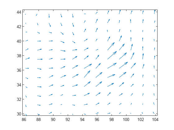
Load sample data that represents air currents over North America. For this example, select a subset of the data.
load('wind','x','y','u','v') X = x(11:22,11:22,1); Y = y(11:22,11:22,1); U = u(11:22,11:22,1); V = v(11:22,11:22,1);
Create a quiver plot of the subset you selected. The vectors X and Y represent the location of the tail of each arrow, and U and V represent the directional components of each arrow. By default, the quiver function shortens the arrows so they do not overlap. Call axis equal to use equal data unit lengths along each axis. This makes the arrows point in the correct direction.
quiver(X,Y,U,V) axis equal
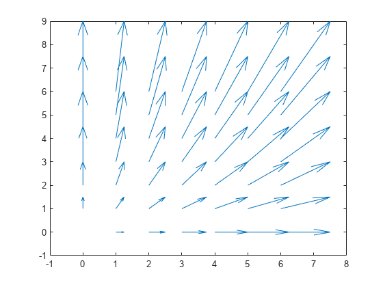
By default, the quiver function shortens arrows so they do not overlap. Disable automatic scaling so that arrow lengths are determined entirely by U and V by setting the scale argument to 0 .
For instance, create a grid of X and Y values using the meshgrid function. Specify the directional components using these values. Then, create a quiver plot with no automatic scaling.
[X,Y] = meshgrid(0:6,0:6); U = 0.25*X; V = 0.5*Y; quiver(X,Y,U,V,0)
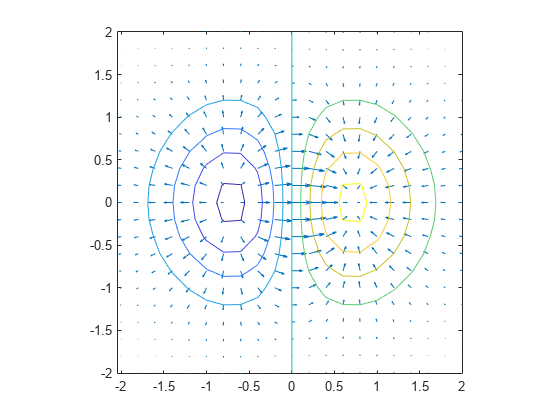
Plot the gradient and contours of the function z = x e - x 2 - y 2 . Use the quiver function to plot the gradient and the contour function to plot the contours.
First, create a grid of x- and y- values that are equally spaced. Use them to calculate z . Then, find the gradient of z by specifying the spacing between points.
spacing = 0.2; [X,Y] = meshgrid(-2:spacing:2); Z = X.*exp(-X.^2 - Y.^2); [DX,DY] = gradient(Z,spacing);
Display the gradient vectors as a quiver plot. Then, display contour lines in the same axes. Adjust the display so that the gradient vectors appear perpendicular to the contour lines by calling axis equal .
quiver(X,Y,DX,DY) hold on contour(X,Y,Z) axis equal hold off
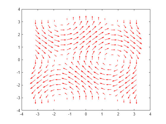
Create a quiver plot and specify a color for the arrows.
[X,Y] = meshgrid(-pi:pi/8:pi,-pi:pi/8:pi); U = sin(Y); V = cos(X); quiver(X,Y,U,V,'r')
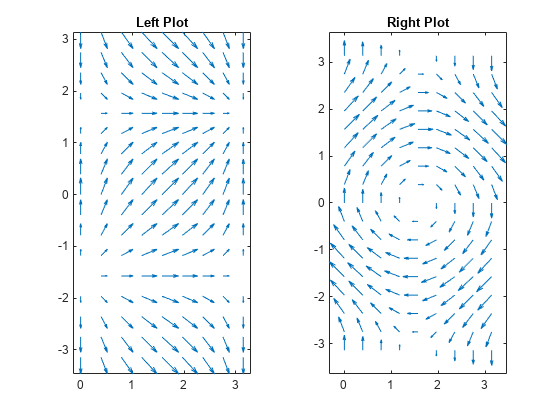
Create a grid of X and Y values and two sets of U and V directional components.
[X,Y] = meshgrid(0:pi/8:pi,-pi:pi/8:pi); U1 = sin(X); V1 = cos(Y); U2 = sin(Y); V2 = cos(X);
Create a tiled layout of plots with two axes, ax1 and ax2 . Add a quiver plot and title to each axes. (Before R2019b, use subplot instead of tiledlayout and nexttile .)
tiledlayout(1,2) ax1 = nexttile; quiver(ax1,X,Y,U1,V1) axis equal title(ax1,'Left Plot') ax2 = nexttile; quiver(ax2,X,Y,U2,V2) axis equal title(ax2,'Right Plot')
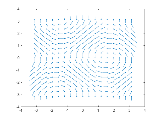
Create a quiver plot and return the quiver object. Then, remove the arrowheads and add dot markers to the end of each tail.
[X,Y] = meshgrid(-pi:pi/8:pi,-pi:pi/8:pi); U = sin(Y); V = cos(X); q = quiver(X,Y,U,V); q.ShowArrowHead = 'off'; q.Marker = '.';
x -coordinates of the arrow tails, specified as a scalar, a vector, or a matrix.
If X and Y are vectors and U and V are matrices, then quiver expands X and Y into matrices. In this case, size(U) and size(V) must equal [length(Y) length(X)] . For more information about expanding vectors into matrices, see meshgrid .
If X and Y are matrices, then X , Y , U , and V must be the same size.
y -coordinates of the arrows tails, specified as a scalar, a vector, or a matrix.
If X and Y are vectors and U and V are matrices, then quiver expands X and Y into matrices. In this case, size(U) and size(V) must equal [length(Y) length(X)] . For more information about expanding vectors into matrices, see meshgrid .
If X and Y are matrices, then X , Y , U , and V must be the same size.
x -components of arrows, specified as a scalar, vector, or matrix.
If X and Y are vectors, then size(U) and size(V) must equal [length(Y) length(X)] .
If X and Y are matrices, then X , Y , U , and V must be the same size.
y -components of arrows, specified as a scalar, vector, or matrix.
If X and Y are vectors, then size(U) and size(V) must equal [length(Y) length(X)] .
If X and Y are matrices, then X , Y , U , and V must be the same size.
Line style, marker, and color, specified as a character vector or string containing symbols. The symbols can appear in any order. You do not need to specify all three characteristics (line style, marker, and color).
If you specify a marker using LineSpec , then quiver does not display arrowheads. To specify a marker and display arrowheads, set the Marker property instead.
Example: '--or' is a red dashed line with circle markers
![]()
![]()
![]()
![]()
![]()
![]()
![]()
![]()
Arrow scaling factor, specified as a nonnegative number or 'off' . By default, the quiver function automatically scales the arrows so they do not overlap. The quiver function applies the scaling factor after it automatically scales the arrows.
Specifying scale is the same as setting the AutoScaleFactor property of the quiver object. For example, specifying scale as 2 doubles the length of the arrows. Specifying scale as 0.5 halves the length of the arrows.
To disable automatic scaling, specify scale as 'off' or 0 . When you specify either of these values, the AutoScale property of the quiver object is set to 'off' and the length of the arrow is determined entirely by U and V .
Target axes, specified as an Axes object. If you do not specify the axes, then the quiver function uses the current axes.
Specify optional pairs of arguments as Name1=Value1. NameN=ValueN , where Name is the argument name and Value is the corresponding value. Name-value arguments must appear after other arguments, but the order of the pairs does not matter.
Before R2021a, use commas to separate each name and value, and enclose Name in quotes.
Example: 'Color','r','LineWidth',1
Note
The properties listed here are only a subset. For a complete list, see Quiver Properties .
Width of arrow stem and head, specified as a scalar numeric value greater than zero in point units. One point equals 1/72 inch. The default value is 0.5 point.
Example: 0.75
Arrowhead display, specified as 'on' or 'off' , or as numeric or logical 1 ( true ) or 0 ( false ). A value of 'on' is equivalent to true , and 'off' is equivalent to false . Thus, you can use the value of this property as a logical value. The value is stored as an on/off logical value of type matlab.lang.OnOffSwitchState .
Use the automatic scale factor to adjust arrow length, specified as 'on' or 'off' , or as numeric or logical 1 ( true ) or 0 ( false ). A value of 'on' is equivalent to true , and 'off' is equivalent to false . Thus, you can use the value of this property as a logical value. The value is stored as an on/off logical value of type matlab.lang.OnOffSwitchState .
Automatic scale factor, specified as a scalar. The automatic scale factor is a multiplier that adjusts the magnitudes of the arrows if the AutoScale property is "on" . For example, a value of 2 doubles the length of the arrows, and a value of 0.5 halves the length of the arrows.
Note
To create a quiver plot using polar coordinates, first convert them to Cartesian coordinates using the pol2cart function.
Usage notes and limitations:
For more information, see Run MATLAB Functions on a GPU (Parallel Computing Toolbox) .
Usage notes and limitations:
For more information, see Run MATLAB Functions with Distributed Arrays (Parallel Computing Toolbox) .
Introduced before R2006a